Introduction to Engineering Computing Skills
EG1004 Lab 1: Software for Engineers I
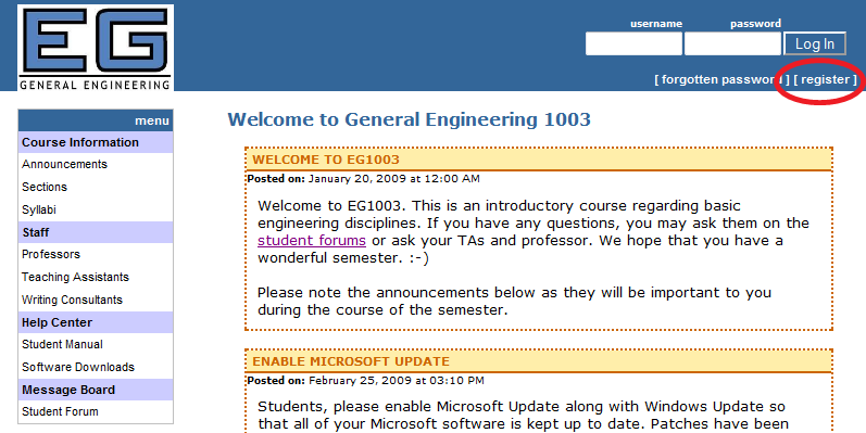
Important: Please note before performing the lab you must register on the EG1004 Web site.
- Click on the register button as shown on the following screen:
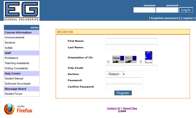
- Fill in the appropriate information on the form that pops up and submit it, as shown on the following screen:
1 OBJECTIVES
The objective of this lab is to use Microsoft Word, Excel, and PowerPoint to perform specific exercises and learn which programs are best suited to particular tasks. Your goal, after having completed the assigned tasks, is to have a basic familiarity with these three software tools.
2 OVERVIEW
This lab is designed to introduce you to three Microsoft applications: Word, Excel, and PowerPoint. Mastering these programs is essential for you to complete your assignments in EG 1004. These software tools are widely used in academic settings as well as in business and industry. Many of you may already be familiar with some of the things they can do. The following exercises are designed to ensure you have a well defined set of basic skills, so please complete all the required tasks.
Microsoft Word
Microsoft Word is a word processing program; its function is to help you create and edit text. It has features that make the mechanics of technical writing relatively easy, but it also has features that make academic dishonesty and plagiarism very easy, too. You are expected to do all the exercises and assignments for this (and all other courses) yourself, unless you are specifically told otherwise, e.g., when you do a team report.
You can create tables and write equations in Word. It also has spelling and grammar checkers and a thesaurus to help you eliminate mistakes in your writing. But beware: running spelling and grammar checks does not eliminate the need for careful editing of all your documents. As powerful as these tools are, they are not foolproof.
In this course, you will use Word to write lab reports and proposals. The thesaurus allows you to quickly find synonyms, so that you can avoid boring repetition in your writing. To use the thesaurus, put the cursor anywhere within the word for which you would like to find a synonym. Pull down the Tools menu and select Language, then Thesaurus. You can also right-click on the word and select Synonyms.
Microsoft Excel
Data collection, manipulation, and analysis are critical steps in the research and design phases of any project. Data can come from a variety of sources including experiments and design calculations. Microsoft Excel, a spreadsheet program, allows you to compile and analyze your data in a systematic fashion.
Excel has many features that streamline data analysis. You can use it to generate tables, charts, and graphs. Excel includes formatting tools, editing features, built-in functions, data manipulation capabilities, and graphing features. It is especially useful for uncovering the relationships that exist between data and to identify trends. You will use it to create graphical elements that will be embedded in your reports, proposals, and presentations.
Microsoft PowerPoint
Microsoft PowerPoint is a presentation program; its function is to create slides for presentations. Presenting information has always been intrinsic to engineering projects. Product introductions, requests for funding, progress reports, and reports to management are just some examples of occasions where presentation skills are required by technical professionals.
Remember, PowerPoint is a tool that will help you make better presentations. It is not a substitute for the longstanding rules to which good public speakers have always adhered. It is most effective when you use it to illustrate the points you want your audience to understand. In EG, you will use PowerPoint to report on your lab work and to present your progress on your Independent Project.
These software tools are essential to your success in EG and beyond. This lab is designed to help you master them by having you perform a specific set of tasks.
3 YOUR ASSIGNMENT
Individual Lab Report
There is no formal write-up for this lab report. Instead, you will submit:
- A title page
- Your MS Word exercise (personalized schedule and non-personalized schedule)
- Your MS Excel exercise (table and graph). Submit the Excel file, which has an .xls file extension, by itself, not as part of a Word document.
Note: The title page and MS Word exercise should be in a single Word document, with the title page and exercise separated by page breaks. (To make a page break, put the cursor where you want a page break, and select Insert/Break. On the popup menu, select Page Break if it's not already selected, and click OK.
IMPORTANT Submit your report electronically using the EG 1004 website: http://eg.poly.edu. You will need to login and upload the lab report material. Submission instructions, a sample coversheet, and a calendar showing the deadlines for your section are located on the website.
4 MATERIALS AND EQUIPMENT
- Lab PC
- Microsoft Office Suite
Remember: You are required to take notes in lab. Experimental details are easily forgotten unless written down. You should keep a laboratory notebook for this purpose. Each week, you must hand in a copy of your lab notes for the Writing Consultant (WC) to review. Keeping careful notes is an essential component of all scientific practice.
However, for this lab only, you are not required to take lab notes, or submit them for review by the Writing Consultant.
5 PROCEDURE
Microsoft Word
Most software has a built-in reference manual to help you learn the program. Always look for a Help menu on the toolbar, and use it whenever you are in doubt about how to do something. This, and regularly saving your work, will save you many lost hours over your working lifetime.
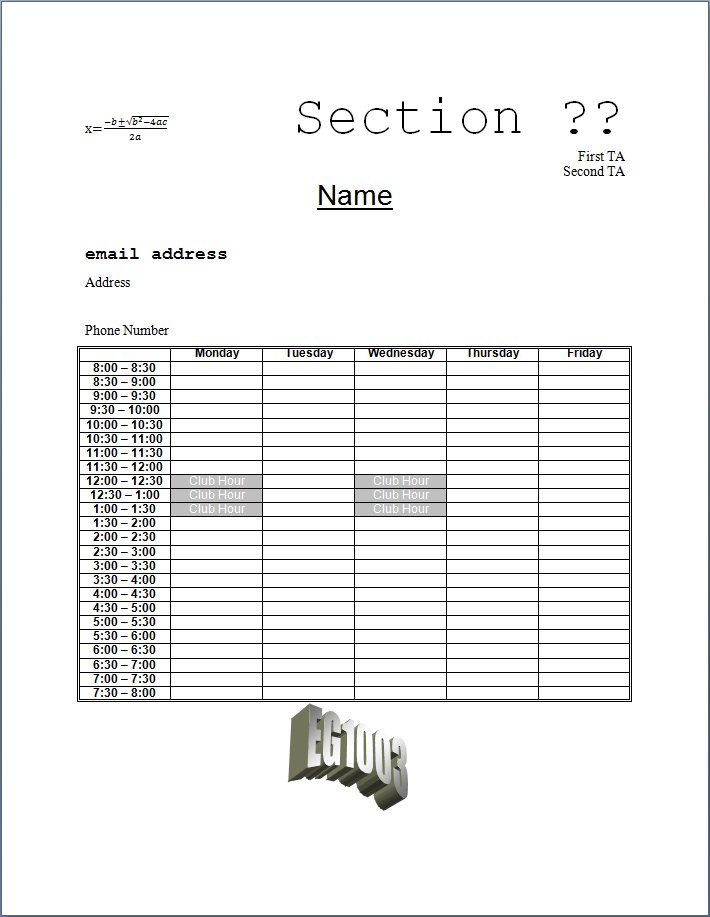
You are going to create two Microsoft Word documents. One will look like Figure 1 below.
Figure 1: Generic Word document
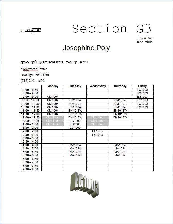
The other will be personalized, and will look like Figure 2.
Figure 2: Personalized Word document
- To open Microsoft Word, go to the Start menu, select Lab Menu then select Lab 1 and click on Microsoft Word.
- On the blank MS Word document page that opens, type the text in quotes below, without including the quotes or the italicized attributes:
- for all text that is aligned right, use single spacing
- for all text that is centered, use double spacing
- for all text that is aligned left, use 1.5-line spacing.
- It is a good idea to periodically save your work. To do this, select Save from the File menu. Name the file “lab01generic.doc�? and save it in the “My Documents�? folder on the lab computer. Later, you must e-mail all the files you create to your personal e-mail account so you can include them in your lab report.
- Now you will insert an equation into the Word document you have created.
- Position the cursor just in front of the word "Section" and left click the mouse. A vertical bar will appear, meaning this is where the equation will be placed.
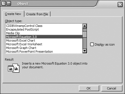
- From the Insert menu select Object. The box shown in Figure 5 will appear.
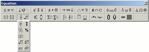
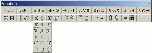
- Select Microsoft Equation 3.0 from the list and click OK. The Equation toolbar shown in Figure 6 will appear.
- To insert the desired quadratic equation in the upper left-hand corner of the page, proceed as follows:
- Select Text from the Style menu and then begin by typing “x=�? (as usual, without the quotes).
- Select the fraction item from the Equation palette (see Figure 7).
- Type “-b�? and then select the plus-or-minus symbol from the Equation palette (see Figure 8).
- Select the radical (square root) symbol from the Equation palette, which is found on the same menu as the fraction item.
- To superscript text (necessary for the “2�? in “b2�?), go to the super/sub script menu on the Equation palette (see Figure 9).
- Complete the expression by typing the remaining characters in the appropriate places. When you are finished, click outside the equation box to return to the ordinary word processing mode.
- Click on the equation and a black frame will appear around it. Right click on the equation, and a drop down menu will appear. Select "Format Object".
- Click on the "Layout" tab, and the picture above "In Front of Text". This will allow you to move the equation around. Click "OK".
- Click and hold down the mouse on the equation. As you move the mouse around, you'll be dragging the equation with you. Drag the equation to the left side of the line and release the mouse. The equation is now where you want it.
- Next, you will insert a table.
- Position the cursor by putting your mouse directly below the "Phone Number" line and clicking it. A vertical bar (the cursor) will appear at the left end of the line.
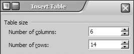
- From the Table menu select Insert, then Table.The box shown in Figure 10 will appear.
- For your Word document, select 6 columns and 14 rows. Make all column and row headings bold and use Arial, 10pt for the text in the table. Center the table on the page. Label the columns with the five days of the week. Label the rows from 8 AM to 9PM. Each row should contain one hour, e.g. 8:00 – 9:00. However, the row should not contain the AM or PM identifiers since the context is obvious.
- Now you will shade the cells and change the borders of your tables. The entire perimeter of each table should have a double-lined border. The Club Hour cells should be shaded.
- Highlight the Club Hour cells (Monday 1:00 pm to 2:00.pm and Wednesday 12:00 noon to 2:00 pm). To highlight an individual cell, place the cursor at the left end of the cell. The cursor will become a black, bolded, angled arrow. Once this arrow appears, click once to highlight the cell.
- On the Format menu, click Borders and Shading. Click the Shading tab and select 25% gray from the color palette. Highlight 'Club Hours' and change text color to white.
- Now click on the Borders tab. Select the double line from the Style list and then select Table from the Apply to drop-down menu.
- Save the changes that have been made by selecting Save from the File menu.
- Finally, you will learn to use Word Art.
- Place the cursor where you want your object to appear.
- On the Insert menu, select Picture, then Word Art.
- A gallery of choices will appear. Select one that resembles our example. Click OK.
- Type “EG1004�? in the box that appears. Click OK.
- Save the document again.
- Now it is time to personalize your document.
- Select Save As from the File menu. Name the file “lab01personal.doc�? and save it in the “My Documents�? folder on the lab computer.
- Personalize the generic document you just created, keeping the appropriate attributes.
- Save this new file.
It is a good idea to use the plain Times New Roman 12 pt font, with full justification as your default, i.e., your starting font and format. Font and paragraph adjustments are located in the Format menu on the main menu bar, as well as on the formatting toolbar. The paragraph alignment buttons looks like this:
“Section ??�? with the following attributes: Courier New 48pt, aligned right
“First TA�? Times New Roman 12pt, aligned right
“Second TA�? Times New Roman 12pt, aligned right
“Name�? Arial 24pt, underlined, centered
“email address�? Courier New 16pt, bold, aligned left
“Address�? Times New Roman 12pt, aligned left
“Phone Number�? Times New Roman 12pt, aligned left
The attributes should be applied to the typed text using the program menus. The attributes can be selected before you type the appropriate text, or applied afterward by selecting (highlighting) the text and then applying the attributes.
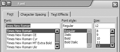
Use the Fonts dialog box, found in the Format menu, to apply the required fonts (see Figure 3).
Figure 3: Fonts dialog box
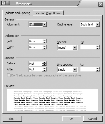
Use the Paragraph dialog box, found in the Format menu, to get the required alignment (see Figure 4).
Figure 4: Paragraph dialog box
Select the line spacing using the Line Spacing menu. Use the following line spacing instructions for your Word document:
Figure 5: Object dialog box
Figure 6: Equation toolbar
Figure 7: Fraction menu
Figure 8: plus-or-minus symbol
Figure 9: super/subscript menu
Figure 10: Insert Table dialog box
To insert a comment (Microsoft Word):
- Put the cursor where you would like the comment inserted.
- Pull down the Insert menu and select Comment.
- Type the text for the comment. You can see the text in the box at the bottom of the screen.
- Click anywhere in the document outside the comment area to finish.
- To delete a comment, right-click on the comment and select Delete Comment.
Microsoft Excel
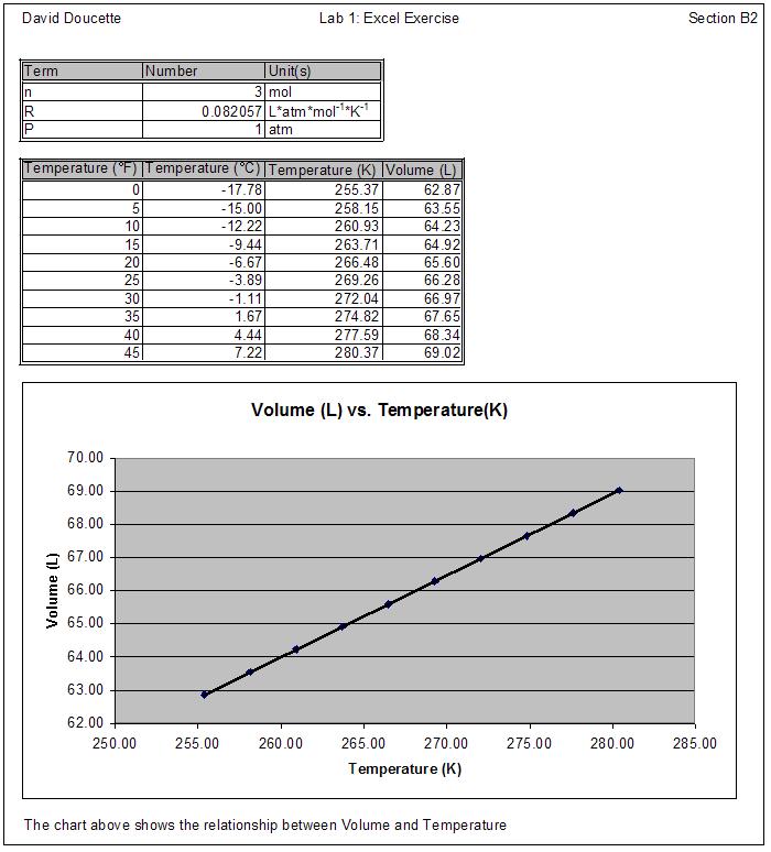
Now you will create a Microsoft Excel document. Your Excel document will include two tables and a graph showing how the volume of a gas changes when its temperature changes. Your Lab TAs will supply each student with a different value for the number of moles, n. The relationship you will graph is known as Charles’ Law. When you are finished, your document will look like Figure 11.
Figure 11: Excel Document
To open Microsoft Excel, go to the Start menu, select Lab Menu then select Lab 1 and click on Microsoft Excel.
Creating a Header
- In the new, blank workbook that opens, select Header and Footer from the View menu and click on the Custom Header button (See Figure 12).
- In the Left section: box type your name. In the Center section: box type “Lab 1: Excel Exercise.�? In the Right section: box type your section. Click "OK" to save this information. Click "OK" again to remove the "Page Setup" window and return to the spreadsheet.
Figure 12: Custom Header dialog box
Note: The Header is not visible on the Excel spreadsheet as you work; it is inserted when the sheet is printed. You can use the Print Preview in the File menu to preview the final document.
Setting up Your Worksheet
To complete the exercise, you will create two tables. The first one is a table of constants. To create it, enter the following information into your Excel worksheet:
- In cell A1, enter Term
- In cell B1 enter Number
- In cell C1 enter Unit(s)
- In cell A2, enter n
- In cell B2, enter the value provided by your TA
- In cell C2, enter mol
- in cell A3, enter R
- In cell B3 enter 0.082057
- In cell C3, enter L*atm*mol-1*K-1
- In cell A4, enter P
- In cell B4, enter 1
- In cell C4, enter atm
To create the superscripted text necessary for cell C3, highlight the text you want superscripted and select Cells from the Format menu. Check the superscript box.
Note:In the next few cells, you'll be inserting the degree symbol. To do this, just type all the text except the degree symbol, and then come back and insert the degree symbol using the instructions in the next note.
Next, you will create a table of computed values. To do this, type the following text into your Excel worksheet:
- In cell A6, enter Temperature (˚F)
- In cell B6, enter Temperature (˚C)
- In cell C6, enter Temperature (K)
- In cell D6, enter Volume (L)
Note: To insert the ˚ symbol, pull down the Insert menu and choose the Symbol Palette. Choose the appropriate symbol and click Insert.
Enter Fahrenheit temperatures 0 – 45 ˚F into cells A7 through A16, increasing the temperature by 5 ˚F in each successive cell.
Using Formulas
Formulas perform calculations in your worksheet. The calculations may use values in other cells, making Excel a very powerful calculator program. A formula is entered in the destination cell where you want the answer to appear. Excel has many built in functions that you can use. The destination cell value is the implied result and so a formula always starts with an equal sign (=).
As an example of the syntax, the formula “= 5*(P98) +ABS(X15)/0.34�? would take the value in cell P98 and multiply it by five, and then add the result to the absolute value of the contents of cell X15 divided by 0.34. If you are in doubt about the order of the mathematical operations, use brackets to make sure the result is calculated correctly. The full range of functions can be selected from the formula menu or by using the fx button on the toolbar.
You will use the following expression to convert your simulated data into degrees Celsius:
- Enter “=5/9*(A7-32)�? into cell B7.
- Copy the formula by dragging the fill handle (solid square on the bottom right of the B7 cell) all the way down to cell B16.
- Click on the cells between B7 and B16 and examine the contents. Notice that the cell reference in the formula has automatically been adjusted in each destination cell.
You will then use the following expression to convert your data into Kelvin:
- Enter “=B7+273.15�? into cell C7.
- Copy the formula into the remaining cells in column C by selecting cell C7 and then dragging the fill handle all the way to cell C16.
- Click on the cell C16 and look at the contents. Notice that the cell reference in the formula (B7) has automatically been adjusted to B16.
You will use the ideal gas law expression to compute the volume for your exercise:
- Enter “=($B$2 *$B$3*C7)/$B$4�? into cell D7.
- Copy the formula into the remaining cells in column D by selecting cell D7 and then dragging the fill handle all the way to cell D16.
- Click on cell D16 and notice that all the cell references except C7 have been kept constant. Typing a $ before a cell reference letter or number fixes the value, even if is it later copied. Two $ keeps both the cell letter and the cell number constant.
Formatting Your Tables
First, you need to be able to see the entire contents of each column. By default, Excel sets all columns to the same width, and fields containing long strings of data can be obstructed by other columns. However, Excel can resize each column to make all the data it contains visible. Always review your data and decide if the number of digits displayed in the worksheet is appropriate.
- Double-click the right edge of the column (see Figure 13).
- In our example two digits after the decimal point is appropriate. Adjust the display by highlighting the data cells B7:D16 and selecting the tab under Cells in the Format menu.
- Select number and two decimal places from the menu. You may also do this by using the increase decimal or decrease decimal buttons on the formatting toolbar.
- Changing the number of places in the "Volume" column now made the column too wide, since it no longer has to hold so many places. Resize the column by double clicking the right edge of the column again.
Figure 13: Column Edge
Creating Table Borders
- In your Excel worksheet, highlight the table of constants (cells A1-C4), and right-click within the highlighted area.
- From the context menu that appears, select Format Cells.
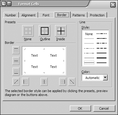
- In the Format Cells dialog box, go to the Border tab.
- Make the constant table professional looking by selecting the double lines in the bottom right corner of the "Style", and the "Outline" preset. Now we'll put grid lines inside by selecting the single line in the bottom left corner of "Style", and the "Inside" present. The preview picture will now show a grid with a double line frame and single line inside lines. Click "OK", and you'll now see the table of constants being nicely framed.
- Next, we'd like to separate the column headers from the numbers. Highlight the column header cells (A1-C1), and right click within the highligted area. Like before, select Format Cells from the context menu that appears and go to the Border tab. Select the double lines in the bottom right corner of "Style" and the "Outline" present. Next, we'd like to shade the column headers so they stand out more. Click on the "Pattern" tab and select the 25% gray box (next to last row on the extreme right side, just above the right box. Click "OK", and you'll see that the column headers now have their own frame and shading.
- Repeat steps 1-5 for the table of computations.
Figure 14: Format Cells dialog box
Creating a Chart
As the final step in this exercise, you will be graphing the relationship between volume and temperature, using the Chart feature in Excel. To create a chart:
- Select the volume values in cells D7–D16.
- Click the Chart Wizard button.

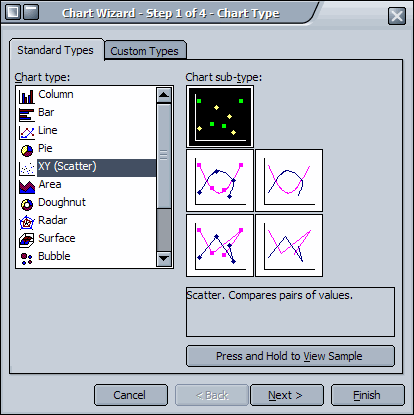
- In the Chart Type dialog box, select XY (Scatter) chart type and leave the chart subtype at the default setting (see Figure 15), then click Next.
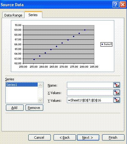
- In the Chart Source dialog box, select the Series tab, as shown in Figure 16.
- Click on the Select From Worksheet button (the icon at the right end of the X Values box). Excel will allow you to select cells directly from your worksheet. Select cells C7–C16 and press Enter.
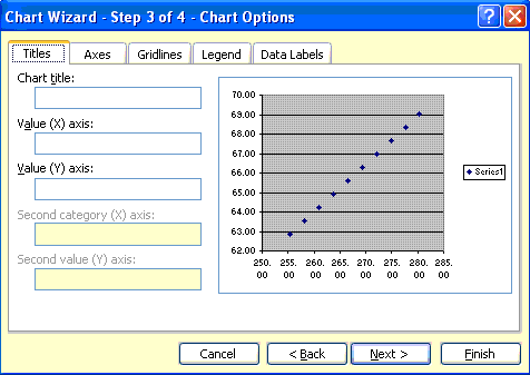
- Click Next and the Chart Options dialog box will appear (see Figure 17
- In the Chart Title: field, enter Volume (L) vs. Temperature (K).
- In the Value(X) axis: field, enter Temperature (K).
- In the Value (Y) axis: field, enter Volume (L).
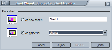
- Click Next and the Chart Location dialog box will appear (see Figure 18).
- In the Chart Location dialog box, select As object in.
- From the drop-down menu, select your current worksheet (see Figure 18).
- Click Finish to create your chart.
- Delete the Series 1 Legend box from your chart. Click on the Legend box and it will be highlighted by having squares on it. Press the delete key to delete the box.
Figure 15: Chart Type dialog box
Figure 16: Chart Source dialog box
Figure 17: Chart Options dialog box
Figure 18: Chart Location dialog box
Adding a Trendline
A trendline is a fit to data, indicating the general behavioral tendency or trend of the data, if any. This allows you to more easily see the nature of any relationship between the quantities in your graph. To add a trendline to your chart:
- Select any data point on your chart. Excel will automatically select all remaining points for you.
- Right-click within the chart. From the context menu that appears, select Add Trendline.
- In the Type tab, select the Linear trend type.
Adding a Caption to Your Chart
- Reposition the chart within your worksheet so that it does not obstruct your data tables. Do this by clicking anywhere on the chart. Squares will appear around the border of the chart indicating that it has been selected. Click the mouse, and "drag" the chart to where you want it, which is typically on the left edge of the spreadsheet, with one row between the bottom of the data table and the top of the chart.
- Select a set of cells beneath your graph roughly the same width as the graph, starting where you want the caption to begin, and right-click within the selected group of cells. From the context menu that appears, select Format Cells.
- In the Alignment tab, check the Wrap Text and Merge Cells checkboxes, and click OK.
- Enter a suitable caption for your chart.
- Save your worksheet as “lab01excel.xls�? and print a copy on a single page.
Microsoft PowerPoint
Now you will create a PowerPoint presentation reporting on the work done in Lab 1. PowerPoint has five viewing windows. Slide View displays one slide at a time, Outline View lists the text for each slide in your presentation, Slide Shorter View displays thumbnails of all your slides allowing you to reorder them easily, and Notes Page View lets you attach text to each slide. Finally, you can view your slides in order in the Slide Show View.
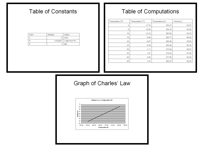
For this lab, your presentation must include a title slide, a brief overview of the presentation, examples of the work done in this lab (either screenshots, or material copied and pasted from the original documents) and a conclusion slide. You may use any design template that you like. Use a title slide at the beginning of your presentation and the bulleted slides for the information that follows. Figure 19 contains some examples of what your slides might look like.
Figure 19: Typical PowerPoint slides
To open Microsoft PowerPoint, go to the Start menu, select Lab Menu then select Lab 1 and click on Microsoft PowerPoint.
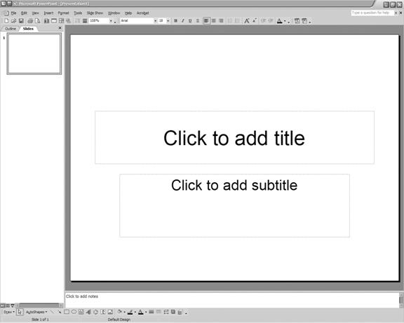
- From the dialog box displayed, select Blank Presentation, or select Blank Presentation from the New Presentation toolbar on the right of the screen. A new slide will appear with the default Title layout (see Figure 20). Click where it says, “Click to add title�? and enter the title of your presentation.
- From the Insert menu, select New Slide (CTRL+M). Click on the new slide. Type the title of the next slide. Click anywhere inside the box marked Click to Add Text and insert your information. Continue this process until you have outlined your entire presentation.
- To add an object from another software application, like Word or Excel, simply copy and paste your object onto the selected PowerPoint slide.
Figure 20: Microsoft PowerPoint, main window. Your screen will look like this when you begin a new presentation.
Microsoft PowerPoint allows you to customize the design of your presentation. You can choose a design template in two ways depending on whether you are just starting your presentation or have already created it.
To select a design template before you begin, select Design Template from the choices that appear when you create a new file. Select the particular design template you would like to use for your presentation.
To select a design template after you start, open the presentation, pull down the Format menu, select Slide Design and apply the design template you like.
Note: With this window open, you can adjust your color schemes, too. After selecting the design template, click on Color Schemes and select the color you like. PowerPoint will apply this color to your template. Remember, a light background with the letters in strong contrast is best.
IMPORTANT
Make sure you run Spell Check when you have completed your presentation! To run it, hit F7. After making any corrections, save your presentation as “lab01PowerPoint.ppt.�?
To print a copy of your PowerPoint Presentation:
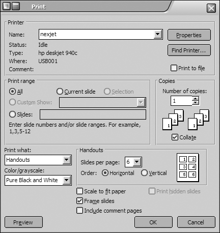
- From the File menu select Print. The box in Figure 21 will appear.
- In the box marked Print what: select Handouts.
- In the box marked Color/grayscale select Pure Black and White.
- In the box marked Slides per page choose six, using Horizontal order.
- Click OK to print.
Figure 21: Microsoft PowerPoint Print dialog box.
Your lab work is now complete. e-mail copies of all the files you created to your personal account. Review the files for errors before submitting your report.
Please clean up your workstation before you leave the lab. Refer to section 3 Your Assignment for the list of the specific items you must submit for your report.
